None
Note
This tutorial was generated from an IPython notebook that can be accessed from github.
3D approximate fractional overlap
This notebook illustrates how the approximate fractional overlap is computed.
Preparation
Import libraries and check the regionmask version:
import cartopy.crs as ccrs
import matplotlib.pyplot as plt
import numpy as np
import shapely

import regionmask

regionmask.__version__
'0.12.1.post1.dev10+g9fd2ed6'
Method
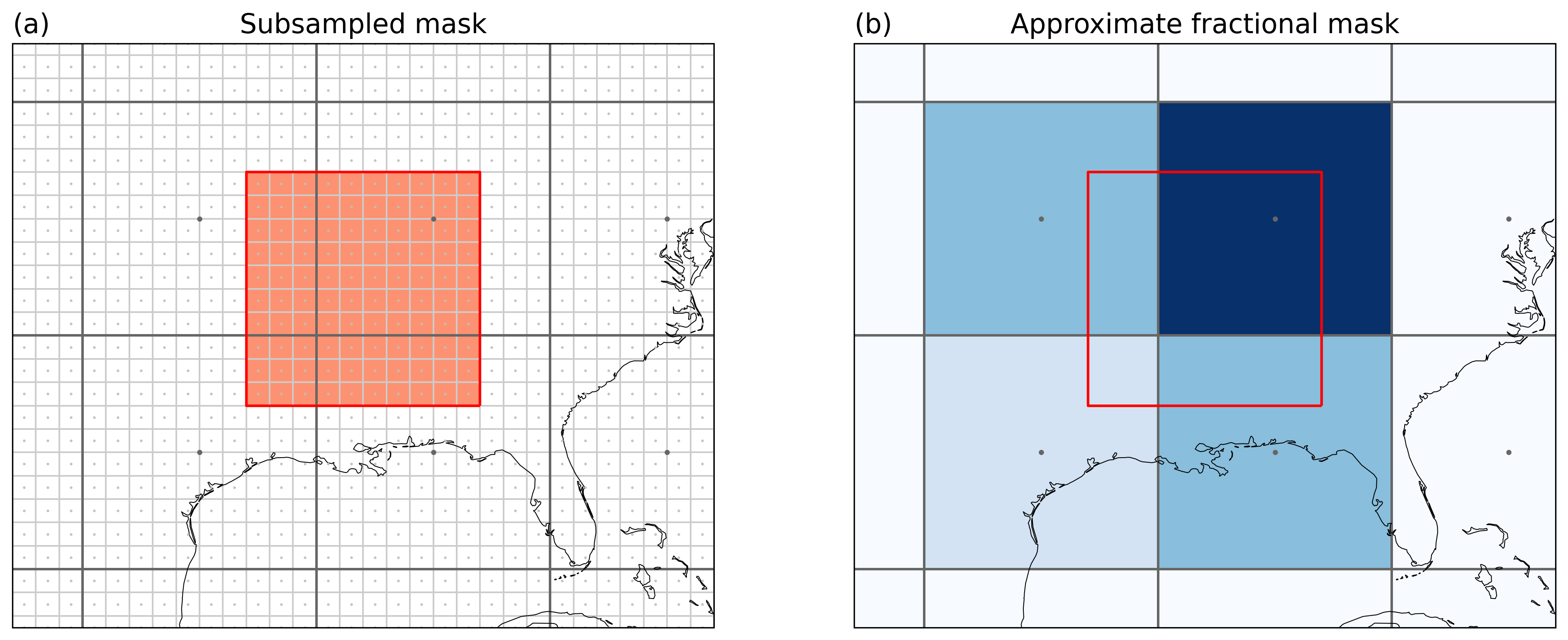
To estimate the approximate fractional overlap, regionmask subsamples each gridpoint. It determines the mask with a grid that is 10 finer than the original one and then averages the subsampled mask to the original one - resulting in a fractional mask. Using this subsampling strategy is considerably faster but combes with some caveats (as also mentioned in the tutorial):
The passed longitude and latitude coordinates must be equally spaced.
Calculating the fractional overlap can be memory intensive.
The resulting mask is correct to about 0.05 or 5%.
Example
Define a region and a lon/ lat grid:
outline = shapely.box(-95, 32, -85, 42)
region = regionmask.Regions([outline])
ds_US = regionmask.core.utils.create_lon_lat_dataarray_from_bounds(
    *(-162, -29, 10), *(75, 13, -10)
)
Manually create the subsampled grid:
ds_US_sub = regionmask.core.utils.create_lon_lat_dataarray_from_bounds(
    *(-162, -29, 1), *(75, 13, -1)
)
Create two masks - once the mask_3D_frac_approx and once from the
subsampled grid to illustrate the method:
mask_frac_approx = region.mask_3D_frac_approx(ds_US)
mask_subsampled = region.mask(ds_US_sub)
Plot the masked regions:
fmt_c = {"ec": "0.4", "lw": 1.0}
fmt_s = {"ec": "0.8", "lw": 0.5}

def plot_grid(ax, ds, **kwargs):
    ax.plot(ds.LON, ds.lat, "o", transform=ccrs.PlateCarree(), **kwargs)

def plot_mask(ax, mask, **kwargs):
    opt = {"add_colorbar": False, "transform": ccrs.PlateCarree()}
    mask.plot(ax=ax, **opt | kwargs)

# ===

f, axs = plt.subplots(1, 2, subplot_kw=dict(projection=ccrs.PlateCarree()))
f.set_size_inches(f.get_size_inches() * 2.5)

ax = axs[0]

plot_mask(ax, mask_subsampled, colors="#fc9272", levels=[0, 1], ec="0.8", lw=0.5)
plot_mask(ax, mask_frac_approx, fc="none", **fmt_c)

plot_grid(ax, ds_US_sub, color="0.75", ms=0.5)


ax = axs[1]
plot_mask(ax, mask_frac_approx, cmap="Blues", **fmt_c)


for ax in axs:
    ax = region.plot_regions(ax=ax, add_label=False, line_kws={"color": "r"})
    ax.set_extent([-105, -75, 22.5, 47.5], ccrs.PlateCarree())
    ax.coastlines(lw=0.5)

    plot_grid(ax, ds_US, color="0.4", ms=2)


axs[0].set_title("Subsampled mask")
axs[1].set_title("Approximate fractional mask")

axs[0].set_title("(a)", loc="left")
axs[1].set_title("(b)", loc="left")

None

Illustrating the method behind mask_3D_frac_approx. Points indicate
the grid cell centers lines the grid cell borders. (a) shows the
original grid (black) and the subsampled grid (light gray). The colored
subsampled grid points belong to the region. (b) Fractional overlap for
the original grid. E.g. the lower left grid cell is at 0.09 (9%) as it
contains 9 / 100 of the subsampled grid points.
The fractional mask is only approximate
Because a subsampling strategy is chosen, the resulting mask is only approximate. We create three regions and a grid to demonstrate this.
# region 1 -> triangle
poly = shapely.geometry.Polygon([[0, 10], [10, 0], [10, 0], [10, 10]])
region1 = regionmask.Regions([poly])

# region 2 -> three quarters of the grid cell
poly = shapely.box(0, 0, 10, 7.5)
region2 = regionmask.Regions([poly])

# region 3 -> 32 % of the gridcell
poly = shapely.box(0, 0, 10, 3.2)
region3 = regionmask.Regions([poly])

regions = [region1, region2, region3]
expected = [0.50, 0.75, 0.32]
lon, lat = np.array([-5, 5, 15]), np.array([-5, 5, 15])
LON, LAT = np.meshgrid(lon, lat)

lons, lats = np.arange(0.5, 10, 1), np.arange(0.5, 10, 1)
LONS, LATS = np.meshgrid(lons, lats)
Illustrate the regions and compare the expected and computed overlap:
cmap = plt.get_cmap("Reds")
cmap.set_under("w")
line_kws = {"color": "#4292c6", "zorder": 4, "lw": 2}
labels = ("a", "b", "c")

# =================

f, axs = plt.subplots(1, 3, sharex=True, sharey=True)
f.set_size_inches(15, 5)

for i, (ax, region, exp, lbl) in enumerate(zip(axs, regions, expected, labels)):

    # create mask
    mask_frac = region.mask_3D_frac_approx(lon, lat).squeeze()
    mask_subsampled = region.mask_3D(lons, lats)


    # plot fractional overlap and region outline
    mask_frac.plot(ax=ax, cmap=cmap, vmax=1, vmin=0.1, add_colorbar=False, lw=1, ec="0.4")
    region.plot_regions(ax=ax, add_label=False, line_kws=line_kws)


    mask_subsampled.plot(ax=ax, colors=["#ffffff00", "#77777744"], levels=[0.5, 1.5], add_colorbar=False)

    # plot the gricell and subsampled gridcell centers
    ax.plot(LON, lat, "o", color="0.4", ms=3, zorder=5)
    ax.plot(LONS, lats, "o", color="0.75", ms=0.5, zorder=5)

    #
    lim = (-1, 11)
    ax.set(title="", xlabel="", ylabel="", xticks=[], yticks=[], xlim=lim, ylim=lim)

    title = f"Expected: {exp:0.2f}, Actual: {mask_frac[1, 1].item():0.2f}"
    ax.set_title(title, loc="right")
    ax.set_title(f"({lbl})", loc="left")

    ax.set_aspect("equal")

    # break

Again, the dark lines and point mark the grid cell. The light grid points mark the subsampled grid cells. The shading indicates the subsampled grid cells that were found to be part of the region. In (a) there is 10 times half a subsampled grid cell missing - resulting in an estimate that is 0.05 too low; (b) has 10 times half a subsampled gridcell too much, thus, overestimating the overlap by 5%, while in (c) 0.2 is missing.
Why not subsample with more points?
It would be possible to get a better estimate of the fractional overlap. However, the precision increases with \(1 / n\), where \(n\) is the number of samples in one dimension, while the total number of points increases as \(n^2\). Thus, a doubling of the precision requires a quadrupling of the number of tested points, which quickly makes it too memory and cpu heavy.