None
Note
This tutorial was generated from an IPython notebook that can be accessed from github.
Matplotlib is building the font cache; this may take a moment.
Edge behavior and interiors
This notebook illustrates the edge behavior (when a grid point falls on the edge of a polygon) and how polygon interiors are treated.
Preparation
Import regionmask and check the version:
import regionmask

regionmask.__version__
'0.10.0'
Other imports
import numpy as np

import cartopy.crs as ccrs
import matplotlib.pyplot as plt

from matplotlib import colors as mplc
from shapely.geometry import Polygon
Define some colors:
color1 = "#9ecae1"
color2 = "#fc9272"

cmap1 = mplc.ListedColormap([color1])
cmap2 = mplc.ListedColormap([color2])

cmap12 = mplc.ListedColormap([color1, color2])
Methods
Regionmask offers two backends (internally called “methods”*) to rasterize regions
rasterize: fastest but only for equally-spaced grid, usesrasterio.features.rasterizeinternally.shapely: for irregular grids, usesshapely.STRtreeinternally.
Note: regionmask offers a third option: pygeos (which is faster than
shapely < 2.0). However, shapely 2.0 replaces pygeos. With shapely 2.0
is is no longer advantageous to install pygeos.
All methods use the lon and lat coordinates to determine if a
grid cell is in a region. lon and lat are assumed to indicate
the center of the grid cell. All methods have the same edge behavior
and consider ‘holes’ in the regions. regionmask automatically
determines which method to use.
and (3) subtract a tiny offset from
lonandlatto achieve a edge behaviour consistent with (1). Due to mapbox/rasterio#1844 this is unfortunately also necessary for (1).
*Note that all “methods” yield the same results.
Edge behavior
The edge behavior determines how points that fall on the outline of a region are treated. It’s easiest to see the edge behaviour in an example.
Example
Define a region and a lon/ lat grid, such that some gridpoints lie exactly on the border:
outline = np.array([[-80.0, 44.0], [-80.0, 28.0], [-100.0, 28.0], [-100.0, 44.0]])

region = regionmask.Regions([outline])
ds_US = regionmask.core.utils.create_lon_lat_dataarray_from_bounds(
    *(-161, -29, 2), *(75, 13, -2)
)

print(ds_US)
<xarray.Dataset>
Dimensions:   (lon: 65, lat: 30, lon_bnds: 66, lat_bnds: 31)
Coordinates:
  * lon       (lon) float64 -160.0 -158.0 -156.0 -154.0 ... -36.0 -34.0 -32.0
  * lat       (lat) float64 74.0 72.0 70.0 68.0 66.0 ... 22.0 20.0 18.0 16.0
  * lon_bnds  (lon_bnds) int64 -161 -159 -157 -155 -153 ... -39 -37 -35 -33 -31
  * lat_bnds  (lat_bnds) int64 75 73 71 69 67 65 63 61 ... 27 25 23 21 19 17 15
    LON       (lat, lon) float64 -160.0 -158.0 -156.0 ... -36.0 -34.0 -32.0
    LAT       (lat, lon) float64 74.0 74.0 74.0 74.0 ... 16.0 16.0 16.0 16.0
Data variables:
    empty
Let’s create a mask with each of these methods:
mask_rasterize = region.mask(ds_US, method="rasterize")
mask_shapely = region.mask(ds_US, method="shapely")
Note
regionmask automatically detects which method to use, so there is no need to specify the method keyword.
Plot the masked regions:
f, axes = plt.subplots(1, 2, subplot_kw=dict(projection=ccrs.PlateCarree()))

opt = dict(add_colorbar=False, ec="0.5", lw=0.5, transform=ccrs.PlateCarree())

mask_rasterize.plot(ax=axes[0], cmap=cmap1, **opt)
mask_shapely.plot(ax=axes[1], cmap=cmap2, **opt)


for ax in axes:
    ax = region.plot_regions(ax=ax, add_label=False)
    ax.set_extent([-105, -75, 25, 49], ccrs.PlateCarree())
    ax.coastlines(lw=0.5)

    ax.plot(
        ds_US.LON, ds_US.lat, "*", color="0.5", ms=0.5, transform=ccrs.PlateCarree()
    )

axes[0].set_title("backend: rasterize")
axes[1].set_title("backend: shapely")
None
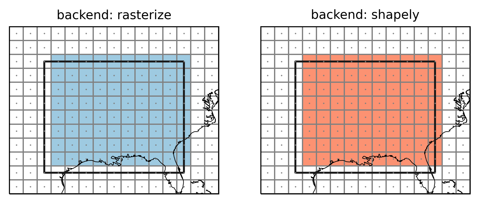
Points indicate the grid cell centers (lon and lat), lines the
grid cell borders, colored grid cells are selected to be part of the
region. The top and right grid cells now belong to the region while the
left and bottom grid cells do not. This choice is arbitrary but follows
what rasterio.features.rasterize does. This avoids spurious columns
of unassigned grid points as the following example shows.
SREX regions
Create a global dataset:
ds_GLOB = regionmask.core.utils.create_lon_lat_dataarray_from_bounds(
    *(-180, 181, 2), *(90, -91, -2)
)
srex = regionmask.defined_regions.srex

srex_new = srex.mask(ds_GLOB)
f, ax = plt.subplots(1, 1, subplot_kw=dict(projection=ccrs.PlateCarree()))

opt = dict(add_colorbar=False, cmap="viridis_r")

srex_new.plot(ax=ax, ec="0.7", lw=0.25, **opt)

srex.plot_regions(ax=ax, add_label=False, line_kws=dict(lw=1))
ax.set_extent([-135, -50, 24, 51], ccrs.PlateCarree())
ax.coastlines(resolution="50m", lw=0.25)

ax.plot(
    ds_GLOB.LON, ds_GLOB.lat, "*", color="0.5", ms=0.5, transform=ccrs.PlateCarree()
)


sel = ((ds_GLOB.LON == -105) | (ds_GLOB.LON == -85)) & (ds_GLOB.LAT > 28)


ax.plot(
    ds_GLOB.LON.values[sel],
    ds_GLOB.LAT.values[sel],
    "*",
    color="r",
    ms=0.5,
    transform=ccrs.PlateCarree(),
)


ax.set_title("edge points are assigned to the left polygon", fontsize=9);
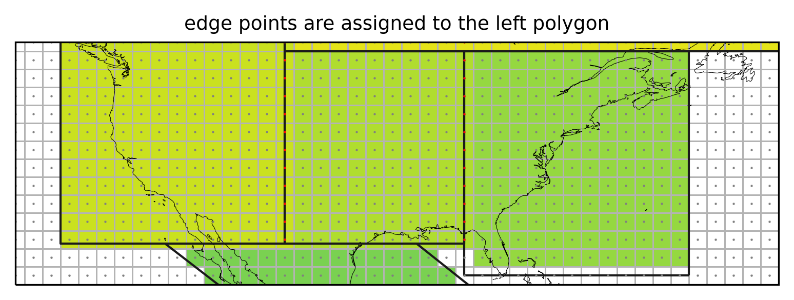
Not assigning the grid cells falling exactly on the border of a region (red points) would leave vertical stripes of unassigned cells.
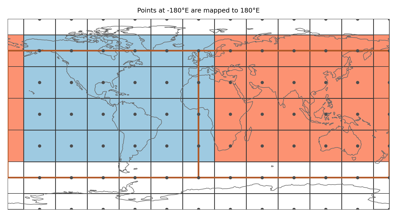
Points at -180°E (0°E) and -90°N
The described edge behaviour leads to a consistent treatment of points on the border. However, gridpoints at -180°E (or 0°E) and -90°N would never fall in any region.
Note
From version 0.8 this applies only if wrap_lon is not set to False. If wrap_lon is set to False regionmask assumes the coordinates are not lat and lon coordinates.
We exemplify this with a region spanning the whole globe and a coarse longitude/ latidude grid:
# almost 360 to avoid wrap-around for the plot
lon_max = 360.0 - 1e-10
outline_global = np.array([[0, 90], [0, -90], [lon_max, -90], [lon_max, 90]])

region_global = regionmask.Regions([outline_global])

lon = np.arange(0, 360, 30)
lat = np.arange(90, -91, -30)

LON, LAT = np.meshgrid(lon, lat)
Create the masks:
# setting `wrap_lon=False` turns this feature off
mask_global_nontreat = region_global.mask(LON, LAT, wrap_lon=False)

mask_global = region_global.mask(LON, LAT)
And illustrate the issue:
proj = ccrs.PlateCarree(central_longitude=180)
f, axes = plt.subplots(1, 2, subplot_kw=dict(projection=proj))
f.subplots_adjust(wspace=0.05)

opt = dict(add_colorbar=False, ec="0.2", lw=0.25, transform=ccrs.PlateCarree())

ax = axes[0]
mask_global_nontreat.plot(ax=ax, cmap=cmap1, x="lon", y="lat", **opt)

ax.set_title("Not treating points at 0°E and -90°N", size=6)
ax.set_title("(a)", loc="left", size=6)

ax = axes[1]
mask_global.plot(ax=ax, cmap=cmap1, x="lon", y="lat", **opt)

ax.set_title("Treating points at 0°E and -90°N", size=6)
ax.set_title("(b)", loc="left", size=6)


for ax in axes:

    ax = region_global.plot(
        ax=ax,
        line_kws=dict(lw=2, color="#b15928"),
        add_label=False,
    )
    ax.plot(LON, LAT, "o", color="0.3", ms=1, transform=ccrs.PlateCarree(), zorder=5)
    ax.spines["geo"].set_visible(False)
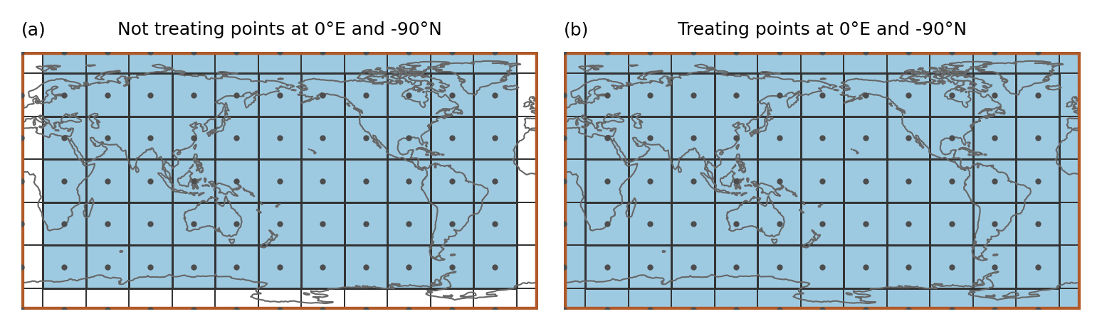
In the example the region spans the whole globe and there are gridpoints at 0°E and -90°N. Just applying the approach above leads to gridpoints that are not assigned to any region even though the region is global (as shown in a). Therefore, points at -180°E (or 0°E) and -90°N are treated specially (b):
Points at -180°E (0°E) are mapped to 180°E (360°E). Points at -90°N are slightly shifted northwards (by 1 * 10 ** -10). Then it is tested if the shifted points belong to any region
This means that (i) a point at -180°E is part of the region that is present at 180°E and not the one at -180°E (this is consistent with assigning points to the polygon left from it) and (ii) only the points at -90°N get assigned to the region above.
This is illustrated in the figure below:
outline_global1 = np.array([[-180.0, 60.0], [-180.0, -60.0], [0.0, -60.0], [0.0, 60.0]])
outline_global2 = np.array([[0.0, 60.0], [0.0, -60.0], [180.0, -60.0], [180.0, 60.0]])

region_global_2 = regionmask.Regions([outline_global1, outline_global2])

mask_global_2regions = region_global_2.mask(lon, lat)
ax = region_global_2.plot(
    line_kws=dict(color="#b15928", zorder=3, lw=1.5),
    add_label=False,
)

ax.plot(
    LON, LAT, "o", color="0.3", lw=0.25, ms=2, transform=ccrs.PlateCarree(), zorder=5
)
mask_global_2regions.plot(ax=ax, cmap=cmap12, **opt)

ax.set_title("Points at -180°E are mapped to 180°E", size=6)

ax.spines["geo"].set_lw(0.25)
ax.spines["geo"].set_zorder(1);
Note
This only applies if the border of the region falls exactly on the point. One way to avoid the problem is to calculate the fractional overlap (see #38) of each gridpoint with the regions (which is not yet implemented).
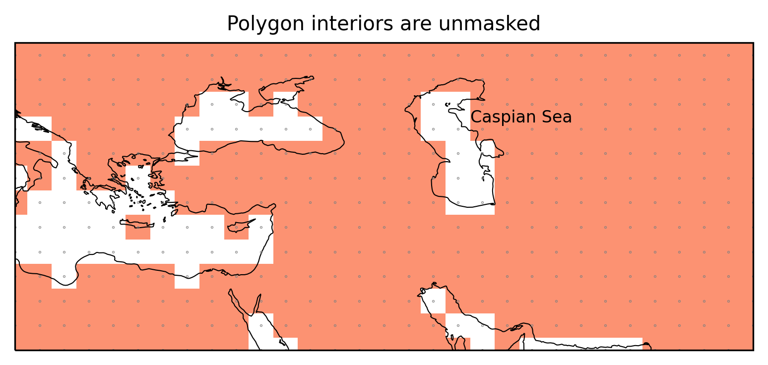
Polygon interiors
Polygons can have interior boundaries (‘holes’). regionmask unmasks
these regions.
Example
Let’s test this on an example and define a region_with_hole:
interior = np.array(
    [
        [-86.0, 40.0],
        [-86.0, 32.0],
        [-94.0, 32.0],
        [-94.0, 40.0],
    ]
)

poly = Polygon(outline, holes=[interior])

region_with_hole = regionmask.Regions([poly])
mask_hole_rasterize = region_with_hole.mask(ds_US, method="rasterize")
mask_hole_shapely = region_with_hole.mask(ds_US, method="shapely")
f, axes = plt.subplots(1, 2, subplot_kw=dict(projection=ccrs.PlateCarree()))

opt = dict(add_colorbar=False, ec="0.5", lw=0.5)

mask_hole_rasterize.plot(ax=axes[0], cmap=cmap1, **opt)
mask_hole_shapely.plot(ax=axes[1], cmap=cmap2, **opt)

for ax in axes:
    region_with_hole.plot_regions(ax=ax, add_label=False, line_kws=dict(lw=1))

    ax.set_extent([-105, -75, 25, 49], ccrs.PlateCarree())
    ax.coastlines(lw=0.25)

    ax.plot(
        ds_US.LON, ds_US.lat, "o", color="0.5", ms=0.5, transform=ccrs.PlateCarree()
    )

axes[0].set_title("backend: rasterize")
axes[1].set_title("backend: shapely")
None
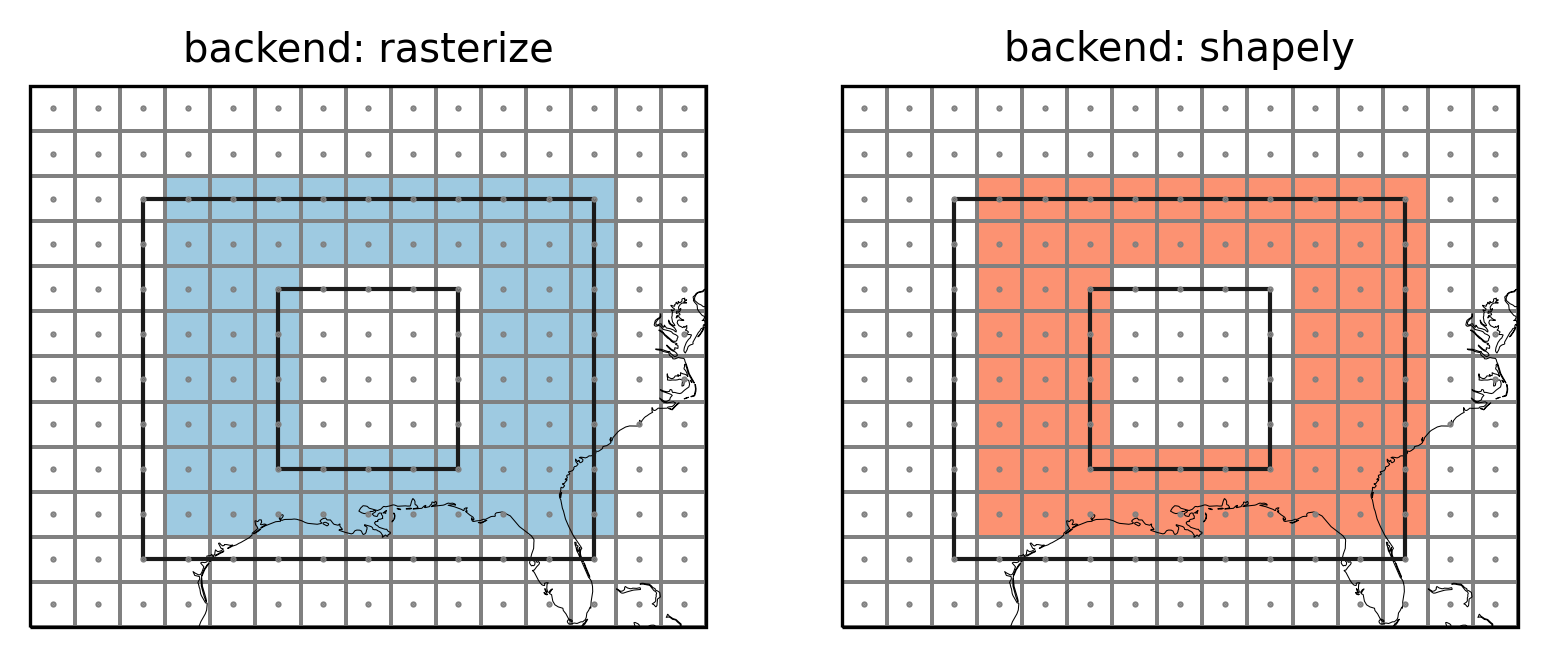
Note how the edge behavior of the interior is inverse to the edge behavior of the outerior.
Caspian Sea
The Caspian Sea is defined as polygon interior.
land110 = regionmask.defined_regions.natural_earth_v5_0_0.land_110

mask_land110 = land110.mask(ds_GLOB)
f, ax = plt.subplots(1, 1, subplot_kw=dict(projection=ccrs.PlateCarree()))

mask_land110.plot(ax=ax, cmap=cmap2, add_colorbar=False)


ax.set_extent([15, 75, 25, 50], ccrs.PlateCarree())
ax.coastlines(resolution="50m", lw=0.5)

ax.plot(
    ds_GLOB.LON, ds_GLOB.lat, ".", color="0.5", ms=0.5, transform=ccrs.PlateCarree()
)


ax.text(52, 43.5, "Caspian Sea", transform=ccrs.PlateCarree())

ax.set_title("Polygon interiors are unmasked");