None

Note

This tutorial was generated from an IPython notebook that can be accessed from github.

Working with geopandas (shapefiles)

regionmask includes support for regions defined as geopandas GeoDataFrame. These are often shapefiles, which can be opened in the formats .zip, .shp, .geojson etc. with geopandas.read_file(url_or_path).

There are two possibilities:

Directly create a mask from a geopandas GeoDataFrame or GeoSeries using mask_geopandas or mask_3D_geopandas.
Convert a GeoDataFrame to a Regions object (regionmask’s internal data container) using from_geopandas.

As always, start with the imports:

import cartopy.crs as ccrs
import geopandas as gp
import matplotlib.pyplot as plt
import matplotlib.patheffects as pe
import numpy as np
import pandas as pd
import pooch

import regionmask

regionmask.__version__

'0.10.0'

Opening an example shapefile

The U.S. Geological Survey (USGS) offers a shapefile containing the outlines of continens [1]. We use the library pooch to locally cache the file:

file = pooch.retrieve(
    "https://pubs.usgs.gov/of/2006/1187/basemaps/continents/continents.zip", None
)

continents = gp.read_file("zip://" + file)

display(continents)

Downloading data from 'https://pubs.usgs.gov/of/2006/1187/basemaps/continents/continents.zip' to file '/home/docs/.cache/pooch/7dd514faeaa71efe73294dece9245e99-continents.zip'.
SHA256 hash of downloaded file: af0ba524a62ad31deee92a9700fc572088c2b93a39ba66f320677dd8dacaaaaf
Use this value as the 'known_hash' argument of 'pooch.retrieve' to ensure that the file hasn't changed if it is downloaded again in the future.

       CONTINENT                                           geometry
         Asia  MULTIPOLYGON (((93.27554 80.26361, 93.31304 80...
North America  MULTIPOLYGON (((-25.28167 71.39166, -25.32889 ...
       Europe  MULTIPOLYGON (((58.06138 81.68776, 57.98055 81...
       Africa  MULTIPOLYGON (((0.69465 5.77337, 0.66667 5.803...
South America  MULTIPOLYGON (((-81.71306 12.49028, -81.72014 ...
      Oceania  MULTIPOLYGON (((-177.39334 28.18416, -177.3958...
    Australia  MULTIPOLYGON (((142.27997 -10.26556, 142.21053...
   Antarctica  MULTIPOLYGON (((51.80305 -46.45667, 51.72139 -...

Create a mask from a GeoDataFrame

mask_geopandas and mask_3D_geopandas allow to directly create a mask from a GeoDataFrame or GeoSeries:

lon = np.arange(-180, 180)
lat = np.arange(-90, 90)

mask = regionmask.mask_geopandas(continents, lon, lat)

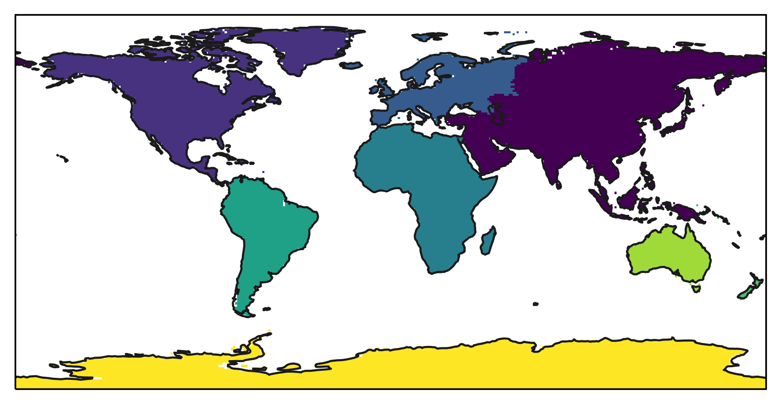
Let’s plot the new mask:

f, ax = plt.subplots(subplot_kw=dict(projection=ccrs.PlateCarree()))
mask.plot(
    ax=ax,
    transform=ccrs.PlateCarree(),
    add_colorbar=False,
)

ax.coastlines(color="0.1");

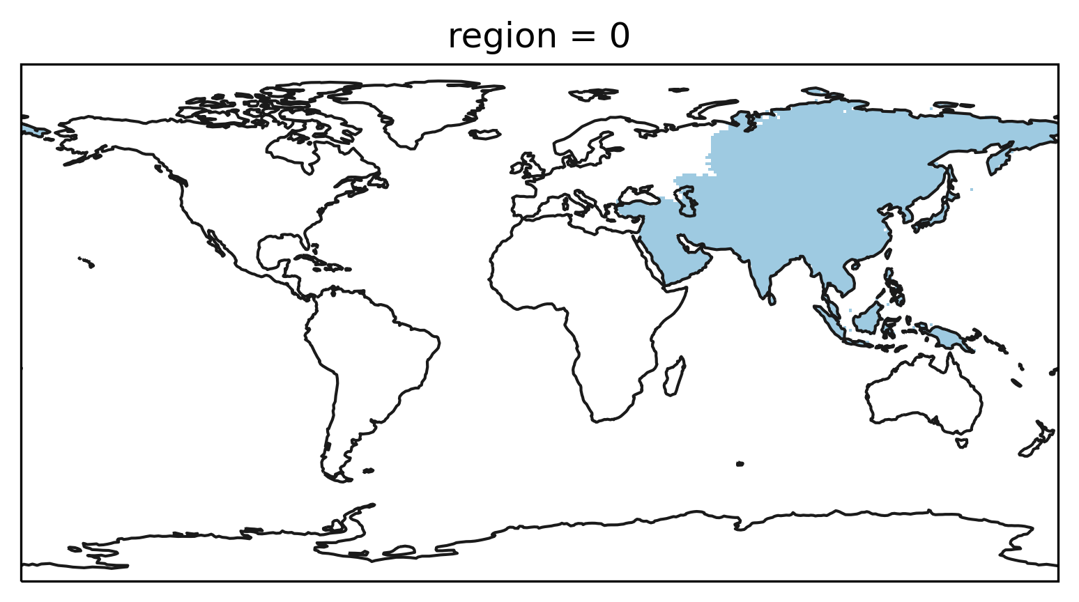
Similarly a 3D boolean mask can be created from a GeoDataFrame:

mask_3D = regionmask.mask_3D_geopandas(continents, lon, lat)

and plotted:

from matplotlib import colors as mplc

cmap1 = mplc.ListedColormap(["none", "#9ecae1"])

f, ax = plt.subplots(subplot_kw=dict(projection=ccrs.PlateCarree()))

mask_3D.sel(region=0).plot(
    ax=ax,
    transform=ccrs.PlateCarree(),
    add_colorbar=False,
    cmap=cmap1,
)

ax.coastlines(color="0.1");

Note

Set regionmask.mask_3D_geopandas(..., overlap=True) if some of the regions overlap. See the tutorial on overlapping regions for details.

2. Convert GeoDataFrame to a Regions object

Creating a Regions object with regionmask.from_geopandas requires a GeoDataFrame:

continents_regions = regionmask.from_geopandas(continents)
continents_regions

<regionmask.Regions 'unnamed'>
overlap:  False

Regions:
0 r0 Region0
1 r1 Region1
2 r2 Region2
3 r3 Region3
4 r4 Region4
5 r5 Region5
6 r6 Region6
7 r7 Region7

[8 regions]

This creates default names ("Region0", …, "RegionN") and abbreviations ("r0", …, "rN").

However, it is often advantageous to use columns of the GeoDataFrame as names and abbrevs. If no column with abbreviations is available, you can use abbrevs='_from_name', which creates unique abbreviations using the names column.

continents_regions = regionmask.from_geopandas(
    continents, names="CONTINENT", abbrevs="_from_name", name="continent"
)
continents_regions

<regionmask.Regions 'continent'>
overlap:  False

Regions:
0    Asi          Asia
1 NorAme North America
2    Eur        Europe
3    Afr        Africa
4 SouAme South America
5    Oce       Oceania
6    Aus     Australia
7    Ant    Antarctica

[8 regions]

Note

Set overlap=True if some of the regions overlap. See the tutorial on overlapping regions for details.

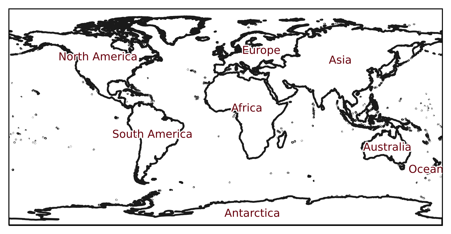
As usual the newly created Regions object can be plotted on a world map:

text_kws = dict(
    bbox=dict(color="none"),
    path_effects=[pe.withStroke(linewidth=2, foreground="w")],
    color="#67000d",
    fontsize=9,
)

continents_regions.plot(label="name", add_coastlines=False, text_kws=text_kws);

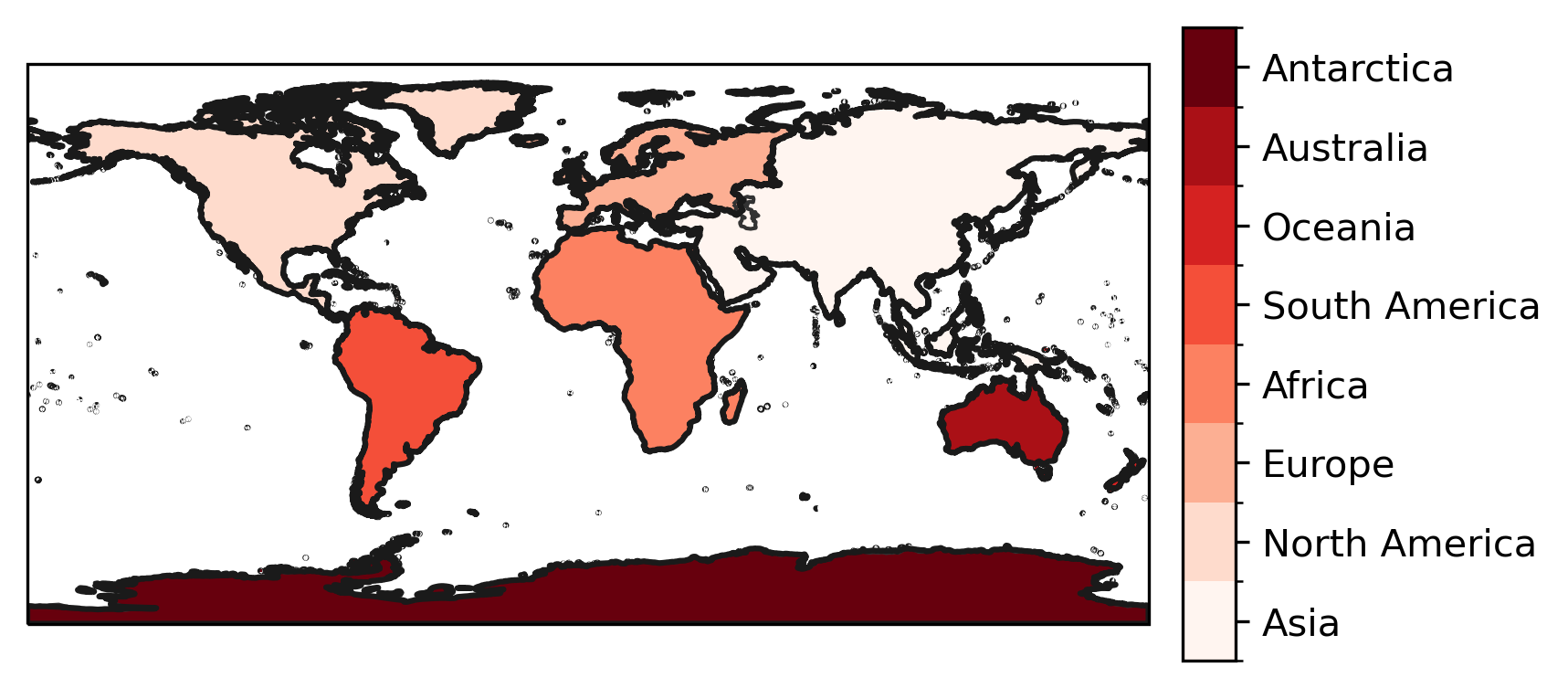
And to create mask a mask for arbitrary latitude/ longitude grids:

lon = np.arange(0, 360)
lat = np.arange(-90, 90)

mask = continents_regions.mask(lon, lat)

which can then be plotted

f, ax = plt.subplots(subplot_kw=dict(projection=ccrs.PlateCarree()))
h = mask.plot(
    ax=ax,
    transform=ccrs.PlateCarree(),
    cmap="Reds",
    add_colorbar=False,
    levels=np.arange(-0.5, 8),
)

cbar = plt.colorbar(h, shrink=0.625, pad=0.025, aspect=12)
cbar.set_ticks(np.arange(8))
cbar.set_ticklabels(continents_regions.names)

ax.coastlines(color="0.2")

continents_regions.plot_regions(add_label=False);

References

[1] Environmental Systems Research , Inc. (ESRI), 20020401, World Continents: ESRI Data & Maps 2002, Environmental Systems Research Institute, Inc. (ESRI), Redlands, California, USA.