None
Note
This tutorial was generated from an IPython notebook that can be accessed from github.
Create 2D integer masks
In this tutorial we will show how to create 2D integer mask for arbitrary latitude and longitude grids.
Note
2D masks are good for plotting. However, to calculate weighted regional averages 3D boolean masks are more convenient. See the tutorial on 3D masks. See GH226 how weighted regional averages can be calculated with 2D integer mask (this may also offer some speed gains).
Import regionmask and check the version:
import regionmask

regionmask.__version__
'0.9.0.post1.dev0+g4000597.d20220302'
Load xarray and the tutorial data:
import xarray as xr
import numpy as np

xr.set_options(display_style="text")
<xarray.core.options.set_options at 0x7fe8ad461750>
Creating a mask
Define a lon/ lat grid with a 1° grid spacing, where the points define the center of the grid.
lon = np.arange(-179.5, 180)
lat = np.arange(-89.5, 90)
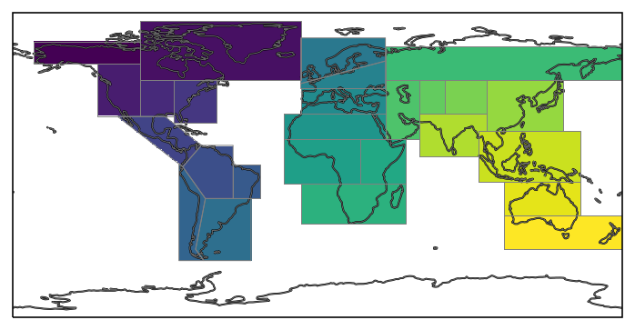
We will create a mask with the SREX regions (Seneviratne et al., 2012).
regionmask.defined_regions.srex
<regionmask.Regions>
Name:     SREX
Source:   Seneviratne et al., 2012 (https://www.ipcc.ch/site/assets/uploads/2...
overlap:  False

Regions:
 1 ALA       Alaska/N.W. Canada
 2 CGI     Canada/Greenl./Icel.
 3 WNA         W. North America
 4 CNA         C. North America
 5 ENA         E. North America
..  ..                      ...
22 EAS                  E. Asia
23 SAS                  S. Asia
24 SEA                S.E. Asia
25 NAU             N. Australia
26 SAU S. Australia/New Zealand

[26 regions]
The function mask determines which gridpoints lie within the polygon
making up the each region:
mask = regionmask.defined_regions.srex.mask(lon, lat)
mask
<xarray.DataArray 'mask' (lat: 180, lon: 360)>
array([[nan, nan, nan, ..., nan, nan, nan],
       [nan, nan, nan, ..., nan, nan, nan],
       [nan, nan, nan, ..., nan, nan, nan],
       ...,
       [nan, nan, nan, ..., nan, nan, nan],
       [nan, nan, nan, ..., nan, nan, nan],
       [nan, nan, nan, ..., nan, nan, nan]])
Coordinates:
  * lat      (lat) float64 -89.5 -88.5 -87.5 -86.5 -85.5 ... 86.5 87.5 88.5 89.5
  * lon      (lon) float64 -179.5 -178.5 -177.5 -176.5 ... 177.5 178.5 179.5
mask is now a xarray.Dataset with shape lat x lon (if you
need a numpy array use mask.values). Gridpoints that do not fall in
a region are NaN, the gridpoints that fall in a region are encoded
with the number of the region (here 1 to 26).
We can now plot the mask:
import cartopy.crs as ccrs
import matplotlib.pyplot as plt

f, ax = plt.subplots(subplot_kw=dict(projection=ccrs.PlateCarree()))
ax.coastlines()

regionmask.defined_regions.srex.plot(
    ax=ax, add_label=False, line_kws=dict(lw=0.5, color="0.5")
)

mask.plot(ax=ax, transform=ccrs.PlateCarree(), add_colorbar=False)
<cartopy.mpl.geocollection.GeoQuadMesh at 0x7fe8acf1fd00>
Working with a mask
masks can be used to select data in a certain region and to calculate regional averages - let’s illustrate this with a ‘real’ dataset:
airtemps = xr.tutorial.load_dataset("air_temperature")
The example data is a temperature field over North America. Let’s plot the first time step:
# choose a good projection for regional maps
proj = ccrs.LambertConformal(central_longitude=-100)

ax = plt.subplot(111, projection=proj)

airtemps.isel(time=1).air.plot.pcolormesh(ax=ax, transform=ccrs.PlateCarree())

ax.coastlines();

Conveniently we can directly pass an xarray object to the mask
function. It gets the longitude and latitude from the DataArray/
Dataset and creates the mask. Per default regionmask assumes the
longitude and latitude are called "lon" and "lat". If they have
another name, you can pass them individually,
e.g. region.mask(ds.longitude, ds.latitude).
mask = regionmask.defined_regions.srex.mask(airtemps)
Note
regionmask automatically detects whether the longitude needs to be wrapped around, i.e. if the regions extend from -180° E to 180° W, while the grid goes from 0° to 360° W as in our example:
lon = airtemps.lon.values
print("Grid extent:    {:3.0f}°E to {:3.0f}°E".format(lon.min(), lon.max()))

bounds = regionmask.defined_regions.srex.bounds_global
print("Region extent: {:3.0f}°E to {:3.0f}°E".format(bounds[0], bounds[2]))
Grid extent:    200°E to 330°E
Region extent: -168°E to 180°E
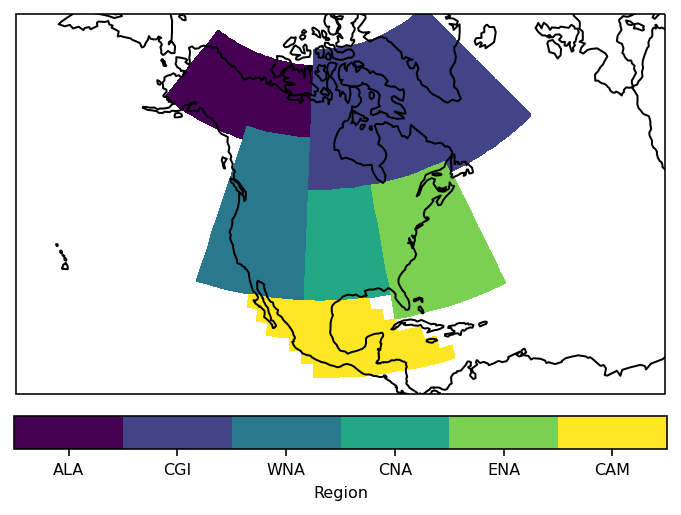
Let’s plot the mask of the regions:
proj = ccrs.LambertConformal(central_longitude=-100)
ax = plt.subplot(111, projection=proj)

low = mask.min()
high = mask.max()

levels = np.arange(low - 0.5, high + 1)

h = mask.plot.pcolormesh(
    ax=ax, transform=ccrs.PlateCarree(), levels=levels, add_colorbar=False
)

# for colorbar: find abbreviations of all regions that were selected
reg = np.unique(mask.values)
reg = reg[~np.isnan(reg)]
abbrevs = regionmask.defined_regions.srex[reg].abbrevs

cbar = plt.colorbar(h, orientation="horizontal", fraction=0.075, pad=0.05)

cbar.set_ticks(reg)
cbar.set_ticklabels(abbrevs)
cbar.set_label("Region")

ax.coastlines()

# fine tune the extent
ax.set_extent([200, 330, 10, 75], crs=ccrs.PlateCarree())
We want to select the region ‘Central North America’. Thus we first need to find out which number this is:
CNA_index = regionmask.defined_regions.srex.map_keys("C. North America")
CNA_index
4
Mask out a region
xarray provides the handy where method
(documentation),
that filters elements from this object according to a condition:
airtemps_CNA = airtemps.where(mask == CNA_index)
Check everything went well by repeating the first plot with the selected region:
# choose a good projection for regional maps
proj = ccrs.LambertConformal(central_longitude=-100)

ax = plt.subplot(111, projection=proj)

regionmask.defined_regions.srex[["CNA"]].plot(ax=ax, add_label=False)

airtemps_CNA.isel(time=1).air.plot.pcolormesh(ax=ax, transform=ccrs.PlateCarree())

ax.coastlines();
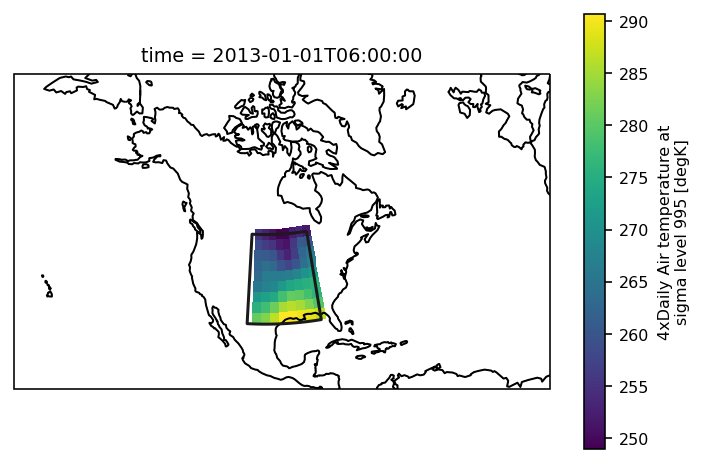
Looks good - with this we can calculate the region average.
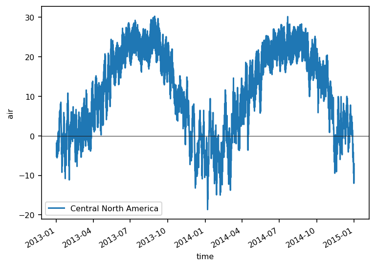
Calculate weighted regional average
From version 0.15.1 xarray includes a function to calculate the weighted
mean - we use cos(lat) as proxy of the grid cell area
Note
It is better to use a model’s original grid cell area (e.g. areacella). cos(lat) works reasonably well for regular lat/ lon grids. For irregular grids (regional models, ocean models, …) it is not appropriate.
weights = np.cos(np.deg2rad(airtemps.lat))

ts_airtemps_CNA = airtemps_CNA.weighted(weights).mean(dim=("lat", "lon")) - 273.15
We plot the resulting time series:
f, ax = plt.subplots()
ts_airtemps_CNA.air.plot.line(ax=ax, label="Central North America")

ax.axhline(0, color="0.1", lw=0.5)

plt.legend();
To get the regional average for each region you would need to loop over them. However, it’s easier to use a 3D mask.
Calculate regional statistics using groupby
Warning
Using groupby offers some convenience and is faster than using where and a loop. However, xarray does currently not natively support to combine groupby with weighted (pydata/xarray#3937), see GH226 for a workaround.
Overall, I recommend working with a 3D mask.
# you can group over all integer values of the mask
airtemps_all = airtemps.groupby(mask).mean()
airtemps_all
<xarray.Dataset>
Dimensions:  (mask: 6, time: 2920)
Coordinates:
  * time     (time) datetime64[ns] 2013-01-01 ... 2014-12-31T18:00:00
  * mask     (mask) float64 1.0 2.0 3.0 4.0 5.0 6.0
Data variables:
    air      (mask, time) float32 255.9 255.7 255.6 254.6 ... 293.8 293.3 294.9
However, groupby is the way to go when calculating a (unweighted)
regional median:
# you can group over all integer values of the mask
airtemps_reg_median = airtemps.groupby(mask).median()
airtemps_reg_median.isel(time=0)
<xarray.Dataset>
Dimensions:  (mask: 6)
Coordinates:
    time     datetime64[ns] 2013-01-01
  * mask     (mask) float64 1.0 2.0 3.0 4.0 5.0 6.0
Data variables:
    air      (mask) float32 255.7 250.8 270.8 269.0 282.9 296.0
Multidimensional coordinates
Regionmask can also handle mutltidimensional longitude/ latitude grids (e.g. from a regional climate model). As xarray provides such an example dataset, we will use it to illustrate it. See also in the xarray documentation.
Load the tutorial data:
rasm = xr.tutorial.load_dataset("rasm")
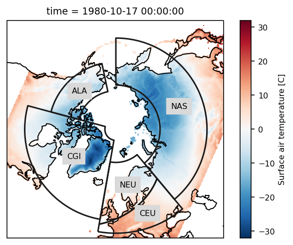
The example data is a temperature field over the Northern Hemisphere. Let’s plot the first time step:
# choose a projection
proj = ccrs.NorthPolarStereo()

ax = plt.subplot(111, projection=proj)
ax.set_global()

rasm.isel(time=1).Tair.plot.pcolormesh(
    ax=ax, x="xc", y="yc", transform=ccrs.PlateCarree()
)

# add the abbreviation of the regions
regionmask.defined_regions.srex[[1, 2, 11, 12, 18]].plot(
    ax=ax, add_coastlines=False, label="abbrev"
)

ax.set_extent([-180, 180, 43, 90], ccrs.PlateCarree())

ax.coastlines();
Again we pass the xarray object to regionmask. We have to pass
rasm.xc and rasm.yc as the longitude and latitude coordinates of
the array:
mask = regionmask.defined_regions.srex.mask(rasm.xc, rasm.yc)
mask
<xarray.DataArray 'mask' (y: 205, x: 275)>
array([[nan, nan, nan, ..., 5., 5., 5.],
[nan, nan, nan, ..., 5., 5., 5.],
[nan, nan, nan, ..., 5., 5., 5.],
...,
[24., 24., 24., ..., 14., 14., 14.],
[24., 24., 24., ..., 14., 14., 14.],
[24., 24., 24., ..., 14., 14., 14.]])
Coordinates:
xc (y, x) float64 189.2 189.4 189.6 189.7 ... 17.65 17.4 17.15 16.91
yc (y, x) float64 16.53 16.78 17.02 17.27 ... 28.26 28.01 27.76 27.51
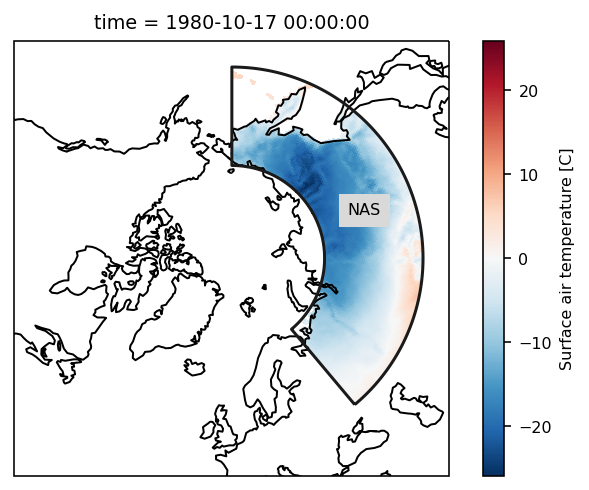
Dimensions without coordinates: y, xWe want to select the region ‘NAS’ (Northern Asia).
Select using where
We have to select by index (the number of the region), we thus map from the abbreviation to the index.
rasm_NAS = rasm.where(mask == regionmask.defined_regions.srex.map_keys("NAS"))
Check everything went well by repeating the first plot with the selected region:
# choose a projection
proj = ccrs.NorthPolarStereo()

ax = plt.subplot(111, projection=proj)
ax.set_global()

rasm_NAS.isel(time=1).Tair.plot.pcolormesh(
    ax=ax, x="xc", y="yc", transform=ccrs.PlateCarree()
)


# add the abbreviation of the regions
regionmask.defined_regions.srex[["NAS"]].plot(
    ax=ax, add_coastlines=False, label="abbrev"
)

ax.set_extent([-180, 180, 45, 90], ccrs.PlateCarree())

ax.coastlines();
References
Special Report on Managing the Risks of Extreme Events and Disasters to Advance Climate Change Adaptation (SREX, Seneviratne et al., 2012)