Note
This tutorial was generated from an IPython notebook that can be downloaded here.
Edge behavior and interiors
This notebook illustrates the edge behavior and how Polygon interiors are treated.
Note
From version 0.5 regionmask treats points on the region borders differently and also considers poygon interiors (holes), e.g. the Caspian Sea in natural_earth.land_110 region.
Preparation
Import regionmask and check the version:
import regionmask

regionmask.__version__
'0.6.0'
Other imports
import xarray as xr
import numpy as np

import cartopy.crs as ccrs
import matplotlib.pyplot as plt

from matplotlib import colors as mplc
from shapely.geometry import Polygon
Define some colors:
cmap1 = mplc.ListedColormap(["#9ecae1"])
cmap2 = mplc.ListedColormap(["#fc9272"])
cmap3 = mplc.ListedColormap(["#cab2d6"])

cmap_2col = mplc.ListedColormap(["#9ecae1", "#fc9272"])
Methods
Regionmask offers three methods to rasterize regions
rasterize: fastest but only for equally-spaced grid, usesrasterio.features.rasterizeinternally.shapely: for irregular grids, usesshapely.vectorized.containsinternally.legacy: old method (deprecated), slowest and with inconsistent edge behaviour
All methods use the lon and lat coordinates to determine if a
grid cell is in a region. lon and lat are assumed to indicate
the center of the grid cell. Methods (1) and (2) have the same edge
behavior and consider ‘holes’ in the regions. Method (3) is deprecated
and will be removed in a future version. regionmask automatically
determines which method to use.
subtracts a tiny offset from
lonandlatto achieve a edge behaviour consistent with (1). Due to mapbox/rasterio/#1844 this is unfortunately also necessary for (1).
Edge behavior
As of version 0.5 regionmask has a new edge behavior - points that
fall of the outline of a region are now consistently treated. This was
not the case in earlier versions (xref
matplotlib/matplotlib#9704).
It’s easiest to see the edge behaviour in an
Example
Define a region and a lon/ lat grid, such that some gridpoints lie exactly on the border:
outline = np.array([[-80.0, 50.0], [-80.0, 28.0], [-100.0, 28.0], [-100.0, 50.0]])

region = regionmask.Regions([outline])
ds_US = regionmask.core.utils.create_lon_lat_dataarray_from_bounds(
    *(-161, -29, 2), *(75, 13, -2)
)

print(ds_US)
<xarray.Dataset>
Dimensions:   (lat: 30, lat_bnds: 31, lon: 65, lon_bnds: 66)
Coordinates:
  * lon       (lon) float64 -160.0 -158.0 -156.0 -154.0 ... -36.0 -34.0 -32.0
  * lat       (lat) float64 74.0 72.0 70.0 68.0 66.0 ... 22.0 20.0 18.0 16.0
  * lon_bnds  (lon_bnds) int64 -161 -159 -157 -155 -153 ... -39 -37 -35 -33 -31
  * lat_bnds  (lat_bnds) int64 75 73 71 69 67 65 63 61 ... 27 25 23 21 19 17 15
    LON       (lat, lon) float64 -160.0 -158.0 -156.0 ... -36.0 -34.0 -32.0
    LAT       (lat, lon) float64 74.0 74.0 74.0 74.0 ... 16.0 16.0 16.0 16.0
Data variables:
    empty
Let’s create a mask with each of these methods:
mask_rasterize = region.mask(ds_US, method="rasterize")
mask_shapely = region.mask(ds_US, method="shapely")
mask_legacy = region.mask(ds_US, method="legacy")
Note
regionmask automatically detects which method to use, so there is no need to specify the method keyword.
Plot the masked regions:
f, axes = plt.subplots(1, 3, subplot_kw=dict(projection=ccrs.PlateCarree()))

opt = dict(add_colorbar=False, ec="0.5", lw=0.5, transform=ccrs.PlateCarree())

mask_rasterize.plot(ax=axes[0], cmap=cmap1, **opt)
mask_shapely.plot(ax=axes[1], cmap=cmap2, **opt)
mask_legacy.plot(ax=axes[2], cmap=cmap3, **opt)


for ax in axes:
    ax = region.plot_regions(ax=ax, add_label=False)
    ax.set_extent([-105, -75, 25, 55], ccrs.PlateCarree())
    ax.coastlines(lw=0.5)

    ax.plot(
        ds_US.LON, ds_US.lat, "*", color="0.5", ms=0.5, transform=ccrs.PlateCarree()
    )

axes[0].set_title("rasterize")
axes[1].set_title("shapely")
axes[2].set_title("legacy");
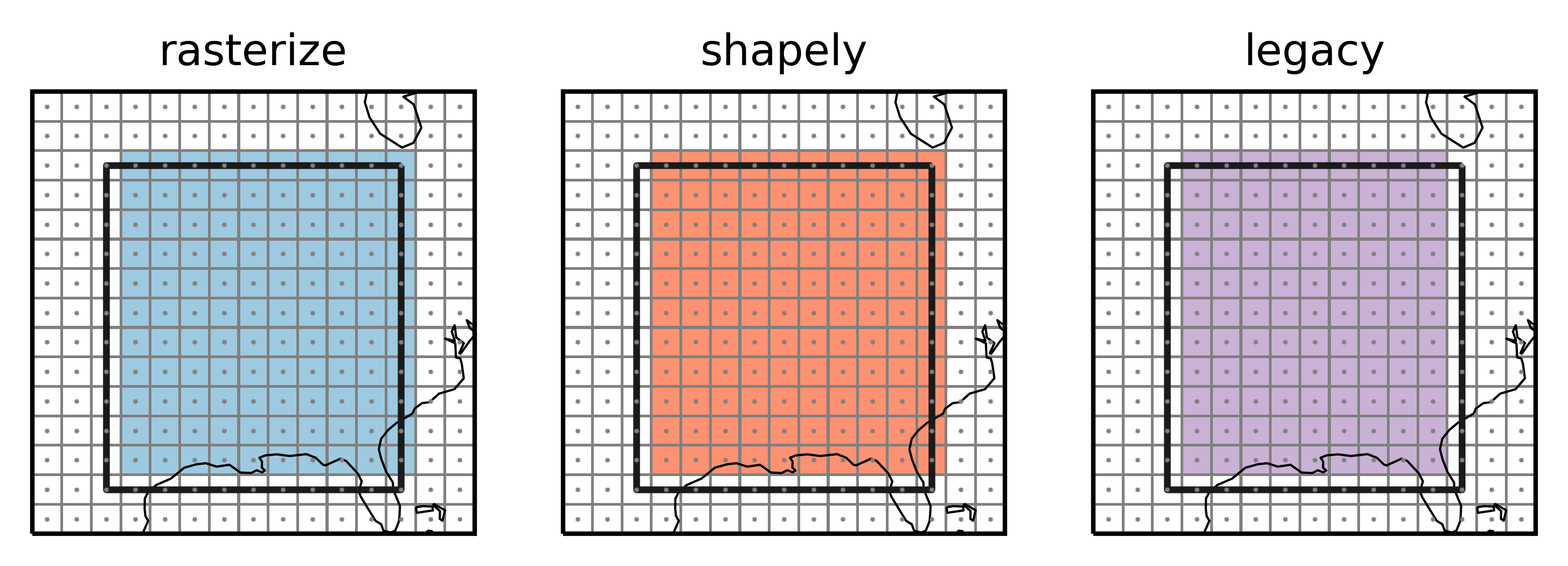
Points indicate the grid cell centers (lon and lat), lines the
grid cell borders, colored grid cells are selected to be part of the
region. The top and right grid cells now belong to the region while the
left and bottom grid cells do not. This choice is arbitrary but mimicks
what rasterio.features.rasterize does. This can avoid spurios
columns of unassigned grid poins as the following example shows.
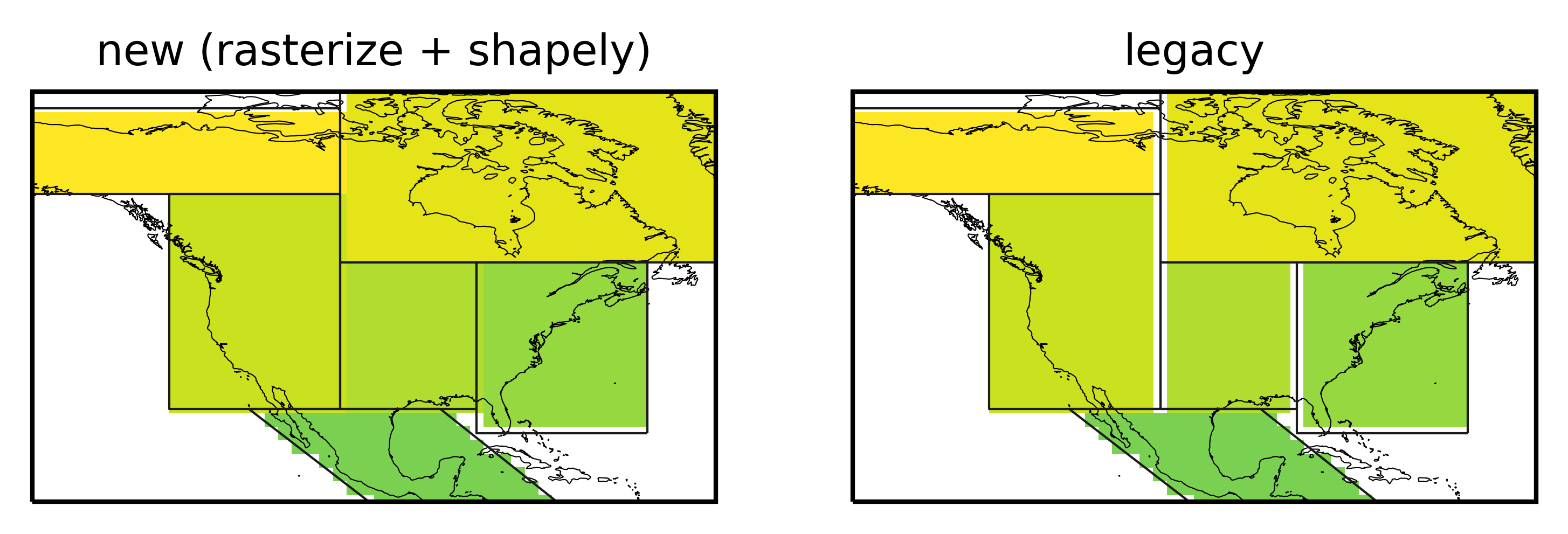
SREX regions
Create a global dataset:
ds_GLOB = regionmask.core.utils.create_lon_lat_dataarray_from_bounds(
    *(-180, 181, 2), *(90, -91, -2)
)
srex = regionmask.defined_regions.srex

srex_new = srex.mask(ds_GLOB)
srex_old = srex.mask(ds_GLOB, method="legacy")
f, axes = plt.subplots(1, 2, subplot_kw=dict(projection=ccrs.PlateCarree()))

opt = dict(add_colorbar=False, cmap="viridis_r")

srex_new.plot(ax=axes[0], **opt)
srex_old.plot(ax=axes[1], **opt)

for ax in axes:
    srex.plot_regions(ax=ax, add_label=False, line_kws=dict(lw=0.5))
    ax.set_extent([-150, -50, 15, 75], ccrs.PlateCarree())
    ax.coastlines(resolution="50m", lw=0.25)

axes[0].set_title("new (rasterize + shapely)")
axes[1].set_title("legacy");
Points at -180°E (0°E) and -90°N
The described edge behaviour leads to a consistent treatment of points on the border. However, gridpoints at -180°E (or 0°E) and -90°N would never fall in any region.
We exemplify this with a region spanning the whole globe and a coarse longitude/ latidude grid:
outline_global = np.array(
    [[-180.0, 90.0], [-180.0, -90.0], [180.0, -90.0], [180.0, 90.0]]
)
region_global = regionmask.Regions([outline_global])

lon = np.arange(-180, 180, 30)
lat = np.arange(90, -91, -30)

LON, LAT = np.meshgrid(lon, lat)
Create the masks:
mask_global = region_global.mask(lon, lat)

# we need to manually create the mask
mask_global_nontreat = mask_global.copy()
mask_global_nontreat[-1, :] = np.NaN
mask_global_nontreat[:, 0] = np.NaN
And illustrate the issue:
f, axes = plt.subplots(1, 2, subplot_kw=dict(projection=ccrs.PlateCarree()))
f.subplots_adjust(wspace=0.05)

opt = dict(add_colorbar=False, ec="0.3", lw=0.5, transform=ccrs.PlateCarree())

ax = axes[0]
mask_global_nontreat.plot(ax=ax, cmap=cmap1, **opt)

# only for the gridlines
mask_global.plot(ax=ax, colors=["none"], levels=1, **opt)

ax.set_title("Not treating points at -180°E and -90°N", size=6)
ax.set_title("(a)", loc="left", size=6)

ax = axes[1]
mask_global.plot(ax=ax, cmap=cmap1, **opt)

ax.set_title("Treating points at -180°E and -90°N", size=6)
ax.set_title("(b)", loc="left", size=6)


for ax in axes:

    ax = region_global.plot(
        ax=ax, line_kws=dict(lw=2, color="#b15928"), add_label=False,
    )
    ax.plot(LON, LAT, "o", color="0.3", ms=2, transform=ccrs.PlateCarree(), zorder=5)

    ax.outline_patch.set_visible(False)
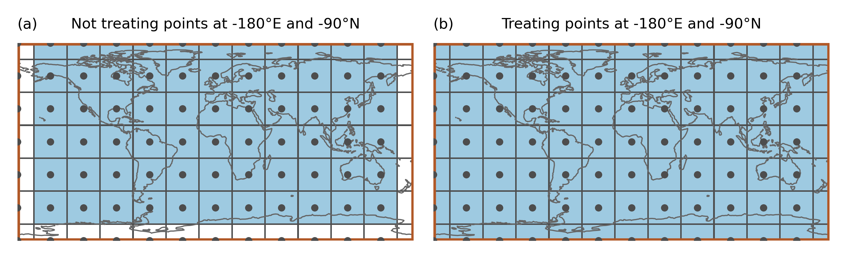
In the example the region spans the whole globe and there are gridpoints at -180°E and -90°N. Just applying the approach above leads to gridpoints that are not assigned to any region even though the region is global (as shown in a). Therefore, points at -180°E (or 0°E) and -90°N are treated specially (b):
Points at -180°E (0°E) are mapped to 180°E (360°E). Points at -90°N are slightly shifted northwards (by 1 * 10 ** -10). Then it is tested if the shifted points belong to any region
This means that (i) a point at -180°E is part of the region that is present at 180°E (and not the one at -180°E) and (ii) only the points at -90°N get assigned to the region above.
outline_global1 = np.array([[-180.0, 60.0], [-180.0, -60.0], [0.0, -60.0], [0.0, 60.0]])
outline_global2 = np.array([[0.0, 60.0], [0.0, -60.0], [180.0, -60.0], [180.0, 60.0]])

region_global_2 = regionmask.Regions([outline_global1, outline_global2])

mask_global_2regions = region_global_2.mask(lon, lat)
ax = region_global_2.plot(line_kws=dict(color="#b15928", zorder=3), add_label=False,)

ax.plot(LON, LAT, "o", color="0.3", ms=2, transform=ccrs.PlateCarree(), zorder=5)

mask_global_2regions.plot(ax=ax, cmap=cmap_2col, **opt)
# only for the gridlines
mask_global.plot(ax=ax, colors=["none"], levels=1, **opt)

ax.set_title("Points at -180°E are mapped to 180°E", size=6)

ax.outline_patch.set_lw(0.5)
ax.outline_patch.set_zorder(1);
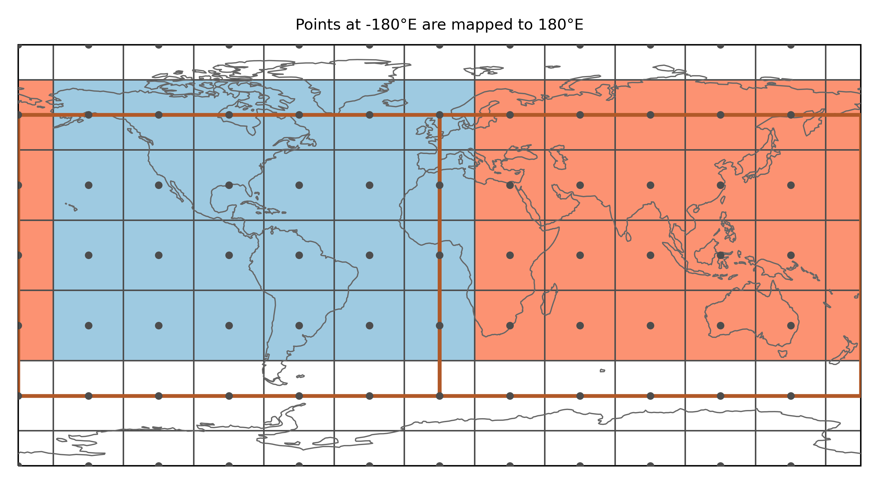
Note
This only applies if the border of the region falls exactly on the point. One way to avoid the problem is to calculate the fractional overlap of each gridpoint with the regions (which is not yet implemented).
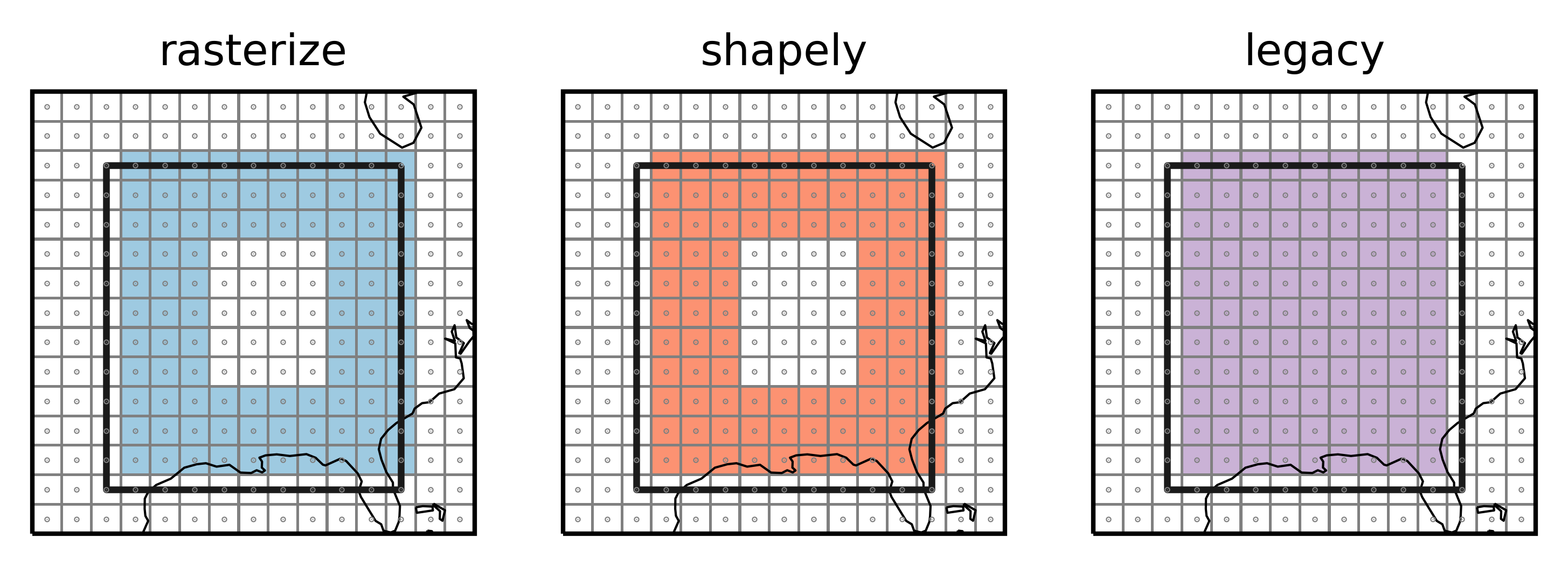
Polygon interiors
Polygons can have interior boundaries (‘holes’). Previously these
were not considered and e.g. the Caspian Sea was not ‘unmasked’.
Example
Let’s test this on an example and define a region_with_hole:
interior = np.array(
    [[-86.0, 44.0], [-86.0, 34.0], [-94.0, 34.0], [-94.0, 44.0], [-86.0, 44.0],]
)

poly = Polygon(outline, [interior])

region_with_hole = regionmask.Regions([poly])
mask_hole_rasterize = region_with_hole.mask(ds_US, method="rasterize")
mask_hole_shapely = region_with_hole.mask(ds_US, method="shapely")
mask_hole_legacy = region_with_hole.mask(ds_US, method="legacy")
f, axes = plt.subplots(1, 3, subplot_kw=dict(projection=ccrs.PlateCarree()))

opt = dict(add_colorbar=False, ec="0.5", lw=0.5)

mask_hole_rasterize.plot(ax=axes[0], cmap=cmap1, **opt)
mask_hole_shapely.plot(ax=axes[1], cmap=cmap2, **opt)
mask_hole_legacy.plot(ax=axes[2], cmap=cmap3, **opt)

for ax in axes:
    region.plot_regions(ax=ax, add_label=False)

    ax.set_extent([-105, -75, 25, 55], ccrs.PlateCarree())
    ax.coastlines(lw=0.5)

    ax.plot(
        ds_US.LON, ds_US.lat, ".", color="0.5", ms=0.5, transform=ccrs.PlateCarree()
    )

axes[0].set_title("rasterize")
axes[1].set_title("shapely")
axes[2].set_title("legacy");
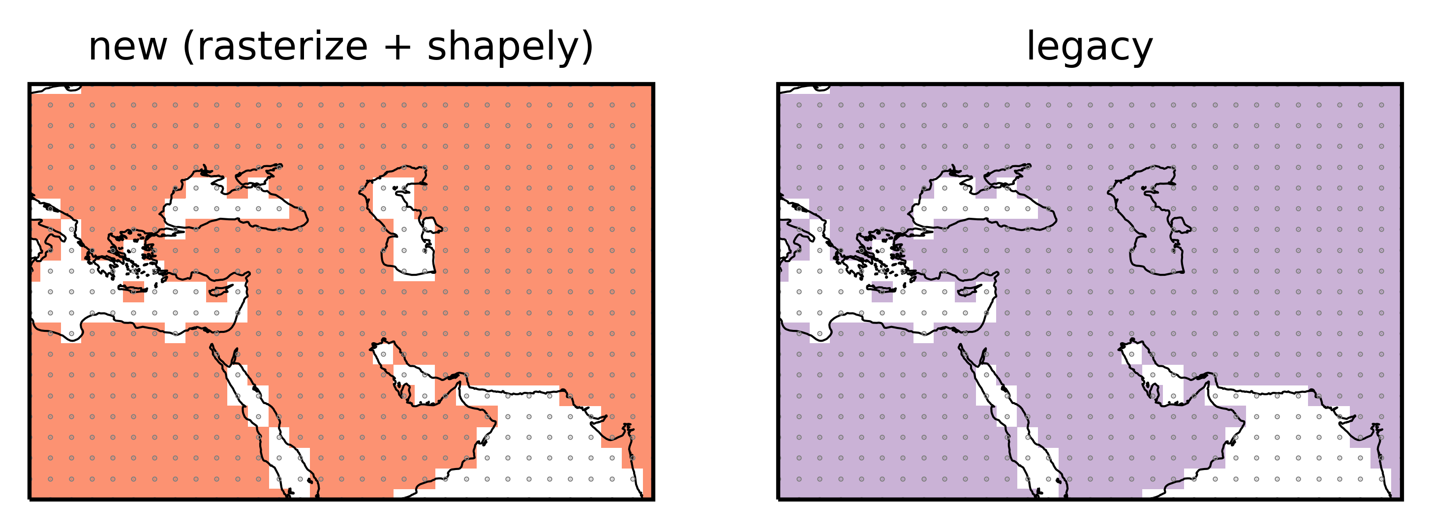
Caspian Sea
land110 = regionmask.defined_regions.natural_earth.land_110

land_new = land110.mask(ds_GLOB)
land_old = land110.mask(ds_GLOB, method="legacy")
f, axes = plt.subplots(1, 2, subplot_kw=dict(projection=ccrs.PlateCarree()))

opt = dict(add_colorbar=False)

land_new.plot(ax=axes[0], cmap=cmap2, **opt)
land_old.plot(ax=axes[1], cmap=cmap3, **opt)

for ax in axes:

    ax.set_extent([15, 75, 15, 55], ccrs.PlateCarree())
    ax.coastlines(resolution="50m", lw=0.5)

    ax.plot(
        ds_GLOB.LON, ds_GLOB.lat, ".", color="0.5", ms=0.5, transform=ccrs.PlateCarree()
    )

axes[0].set_title("new (rasterize + shapely)")
axes[1].set_title("legacy");
Speedup
The new methods are faster than the old one:
print("Method: rasterize")
%timeit -n 10 region.mask(ds_US, method="rasterize")
print("Method: shapely")
%timeit -n 10 region.mask(ds_US, method="shapely")
print("Method: legacy")
%timeit -n 10 region.mask(ds_US, method="legacy")
Method: rasterize
2.28 ms ± 154 µs per loop (mean ± std. dev. of 7 runs, 10 loops each)
Method: shapely
1.66 ms ± 57.4 µs per loop (mean ± std. dev. of 7 runs, 10 loops each)
Method: legacy
3.62 ms ± 147 µs per loop (mean ± std. dev. of 7 runs, 10 loops each)
While there is not a big difference for this simple example, the difference gets larger for more complex geometries and more gridpoints:
ds_GLOB = regionmask.core.utils.create_lon_lat_dataarray_from_bounds(
    *(-180, 181, 2), *(90, -91, -2)
)

countries_110 = regionmask.defined_regions.natural_earth.countries_110
print("Method: rasterize")
%timeit -n 1 countries_110.mask(ds_GLOB, method="rasterize")
Method: rasterize
18.6 ms ± 3.21 ms per loop (mean ± std. dev. of 7 runs, 1 loop each)
print("Method: shapely")
%timeit -n 1  countries_110.mask(ds_GLOB, method="shapely")
Method: shapely
315 ms ± 4.85 ms per loop (mean ± std. dev. of 7 runs, 1 loop each)
print("Method: legacy")
%timeit -n 1  countries_110.mask(ds_GLOB, method="legacy")
Method: legacy
4.85 s ± 46 ms per loop (mean ± std. dev. of 7 runs, 1 loop each)