Note

This tutorial was generated from an IPython notebook that can be downloaded here.

Create xarray region mask¶

In this tutorial we will show how to create a mask for arbitrary latitude and longitude grids using xarray. It is very similar to the tutorial Create Mask (numpy).

Import regionmask and check the version:

import regionmask
regionmask.__version__

'0.9.0'

Load xarray and the tutorial data:

import xarray as xr
import numpy as np

airtemps = xr.tutorial.load_dataset('air_temperature')

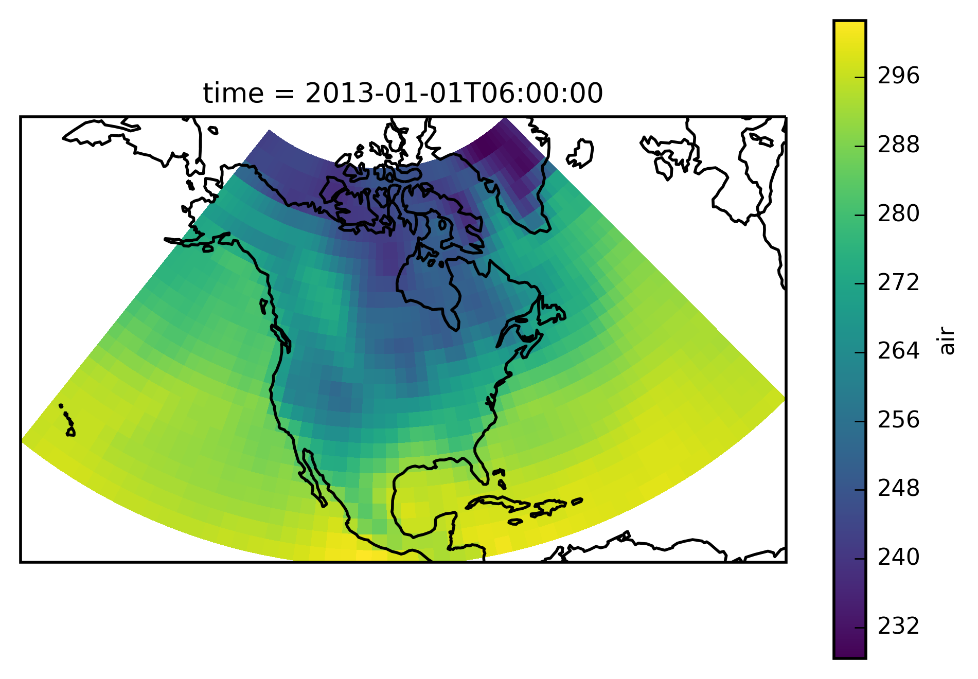
The example data is a temperature field over North America. Let’s plot the first time step:

# load cartopy
import cartopy.crs as ccrs

# choose a good projection for regional maps
proj=ccrs.LambertConformal(central_longitude=-100)

ax = plt.subplot(111, projection=proj)

airtemps.isel(time=1).air.plot.geocolormesh(ax=ax, transform=ccrs.PlateCarree())

ax.coastlines();

/home/mathause/.local/lib/python2.7/site-packages/matplotlib/artist.py:221: MatplotlibDeprecationWarning: This has been deprecated in mpl 1.5, please use the
axes property.  A removal date has not been set.
  warnings.warn(_get_axes_msg, mplDeprecation, stacklevel=1)

Conviniently we can directly pass an xarray object to the mask function. It gets the longitude and latitude from the DataArray/ Dataset and creates the mask. If the longituda and latitude in the xarray object are not called lon and lat, respectively; their name can be given via the lon_name and lat_name keyword. Here we use the Giorgi regions.

mask = regionmask.giorgi.mask(airtemps)
print('All NaN? ',np.all(np.isnan(mask)))

All elements of mask are NaN. Try to set 'wrap_lon=True'.
All NaN?  True

This didn’t work - all elements are NaNs! The reason is that airtemps has its longitude from 0 to 360 while the Giorgi regions are defined as -180 to 180. Thus we can provide the wrap_lon keyword:

mask = regionmask.giorgi.mask(airtemps, wrap_lon=True)
print('All NaN? ',np.all(np.isnan(mask)))

All NaN?  False

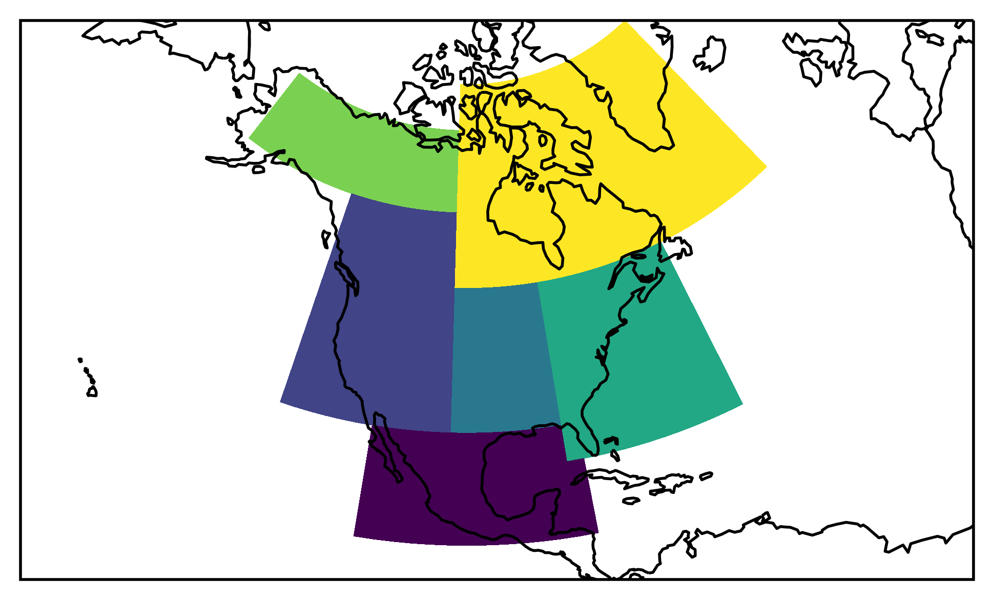
This is better. Let’s plot the regions:

proj=ccrs.LambertConformal(central_longitude=-100)
ax = plt.subplot(111, projection=proj)

low = mask.min()
high = mask.max()

levels = np.arange(low - 0.5, high + 1)

mask.plot.pcolormesh(ax=ax, transform=ccrs.PlateCarree(), levels=levels, add_colorbar=False)

ax.coastlines()

# fine tune the extent
ax.set_extent([200, 330, 10, 75], crs=ccrs.PlateCarree());

We want to select the region ‘Central North America’. Thus we first need to find out which number this is:

regionmask.giorgi.map_keys('Central North America')

xarray provides the handy where function:

airtemps_CNA = airtemps.where(mask == 6)

Check everything went well by repeating the first plot with the selected region:

# choose a good projection for regional maps
proj=ccrs.LambertConformal(central_longitude=-100)

ax = plt.subplot(111, projection=proj)

airtemps_CNA.isel(time=1).air.plot.geocolormesh(ax=ax, transform=ccrs.PlateCarree())

ax.coastlines();

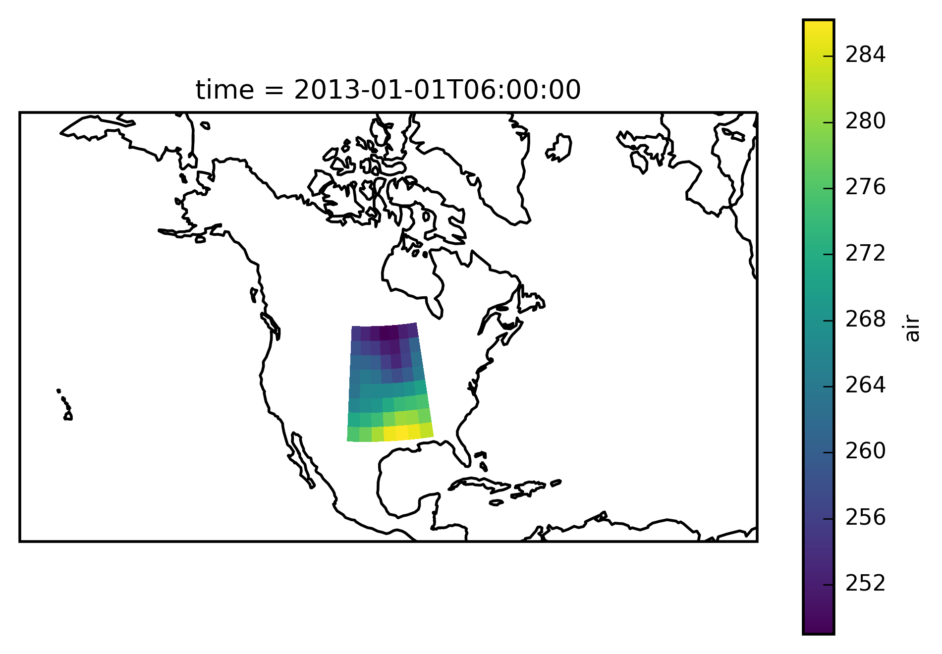
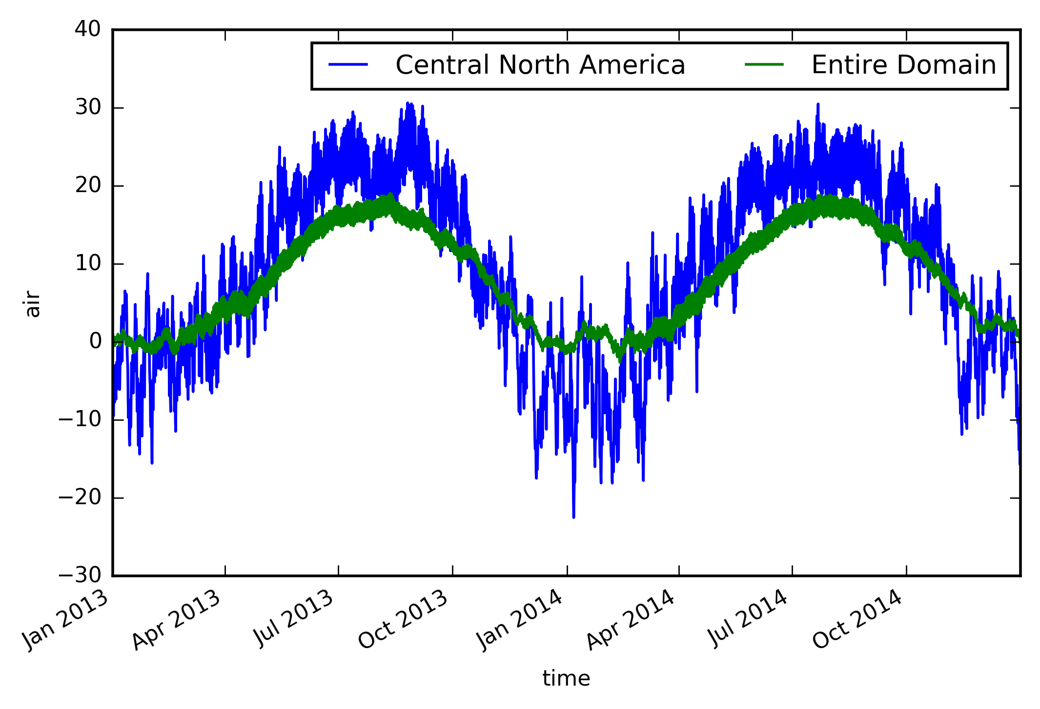
Looks good - let’s take the area average and plot the time series. (Note: you should use cos(lat) weights to correctly calculate an area average. Unfortunately this is not yet (as of version 0.7) implemented in xarray.)

ts_airtemps_CNA = airtemps_CNA.mean(dim=('lat', 'lon')) - 273.15
ts_airtemps = airtemps.mean(dim=('lat', 'lon')) - 273.15

# and the line plot
ts_airtemps_CNA.air.plot.line(label='Central North America')
ts_airtemps.air.plot(label='Entire Domain')

plt.legend(ncol=2)

<matplotlib.legend.Legend at 0x2adada801dd0>